In this blog, we will see how statistical tolerance intervals can be applied to infer the proportion of individual products within a population.
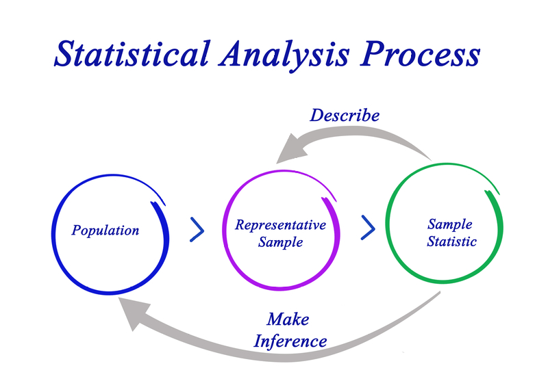
We take a representative sample from a population, compute sample statistics, and make an inference about a population parameter. The most familiar sample statistic is the sample mean. That is used to calculate a confidence interval regarding the location of the population mean, the inference.
However, confidence intervals for the mean are inferring the location of averages. In decision-making, it is often more important to focus on individual values. For that, we have the statistical tolerance interval.
As defined, a statistical tolerance interval infers the location of a given proportion of the individual values at a given level of confidence. For example, suppose we wish to know with 95% confidence, the range of 90% of the individual values for a product based on a random sample. This would be a two-sided interval, the subject of our discussion.
NOTE: One can also calculate one-sided intervals for a minimum or a maximum depending on the nature of the investigation.
Examples of uses include:
- Individual battery lives
- Assay values for drug containers
- Range of a given air pollutant
- Food safety assessment
- Blood pressure levels for a certain percentage of the population for a population segment
- Package burst strength
- Process qualification
As you can imagine, the uses are endless.
The following short video by Keith Bower does a nice job of introducing the concept of statistical tolerance intervals and why you should use them. You can watch Keith’s video here.
Now, after the video, let’s give an example of a two-sided statistical tolerance interval use and calculate the interval using two platforms often used in Six Sigma training: Minitab and SigmaXL. For this presentation we used
- Minitab 17
- SigmaXL 8.13
We are also assuming the data is normally distributed for this simpler example. There are methods available for computing statistical tolerance intervals using a non-parametric approach for non-normal data.
We will use the method developed by Howe in 1969.
Howe, W. G. (1969). "Two-sided Tolerance Limits for Normal Populations - Some Improvements", Journal of the American Statistical Association, 64 , pages 610-620.
The formula to be used is shown in this excerpt from the NIST Engineering Statistics Handbook.

While Guenther provides a w correction factor: w*K2, we will not employ it here in order to match the Minitab and SigmaXL results.
Guenther, W. C. (1977). "Sampling Inspection in Statistical Quality Control", Griffin's Statistical Monographs, Number 37, London.
The Problem: A cereal manufacturer takes a random sample of 100 cereal boxes and weighs them. With 95% confidence, within what range can we expect 90% of the box weights to fall in grams?
Summary Statistics for the Cereal Data:
N = 100
Mean = 589.01
STDEV = 2.04
The data is normally distributed.
Statistical Tolerance Interval Calculation: Minitab 17
Access Tolerance Intervals by Stat > Quality Tools > Tolerance Intervals. Input the summary information as shown.

Now choose options and enter the desired information as shown.

Clicking OK twice, we get the final result.

Weight data is normally distributed, and the cereal box weights are no exception. The nonparametric method does not apply here.
90% of the cereal boxes should range from 585.185 to 592.835 grams with 95% confidence.
Statistical Tolerance Interval Calculation: SigmaXL 8.13
Access the Tolerance Interval Calculator.
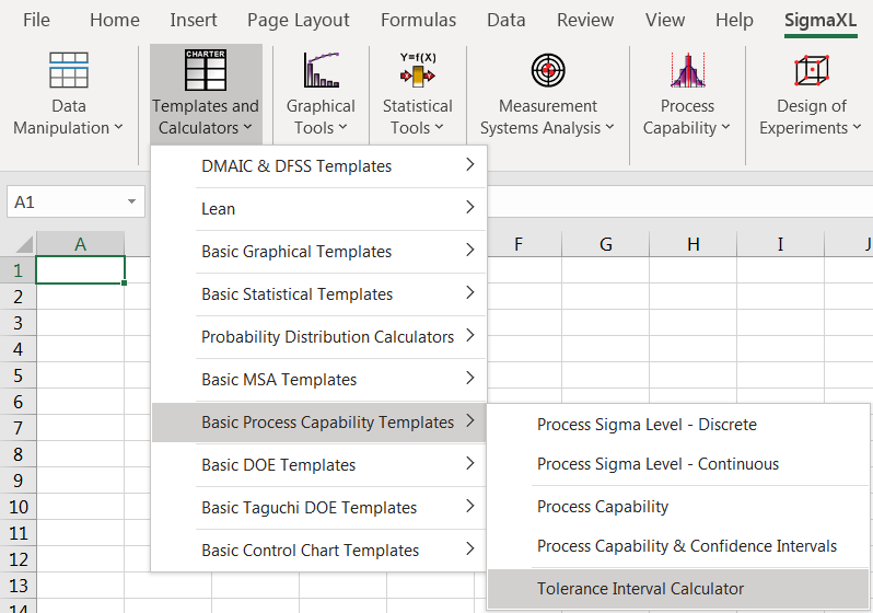
The calculator appears.

Enter the data for our cereal problem.

We obtain identical results: 90% of the boxes weigh from 585.185 to 592.835 grams with 95% confidence.
We hope this short introduction to the use of statistical tolerance intervals will encourage you to use them where appropriate in your projects.


Leave A Comment